DEM Processing Code

written for the Polar Geospatial Center

Project description: Code written for working with DEMs produced by the Polar Geospatial Center. Some functionality is highlighted below”

Create a No Data Mask — valid_data.py

As the PGC uses stereo satellite imagery to create DEMs, there are sometimes areas of No Data in the resulting DEM. This is usually in areas of water, clouds, or shadow, where the point-matching algorithm (the PGC uses SETSM could not locate match points, or post-processing filters removed bad data or artifacts. This script includes a function to open a single band raster using GDAL and identify the areas of No Data. This function returns a count of valid data pixels and a total count so that users can get an idea of the quality of the DEM without needing to load it into a point and click GIS, compute statistics, set visualization, etc. The script includes options to write the valid data areas out as a binary raster.

For example, consider the following area of interest over a glacier terminus that we wish to perform mass balance analysis on (forgive the coarse imagery):

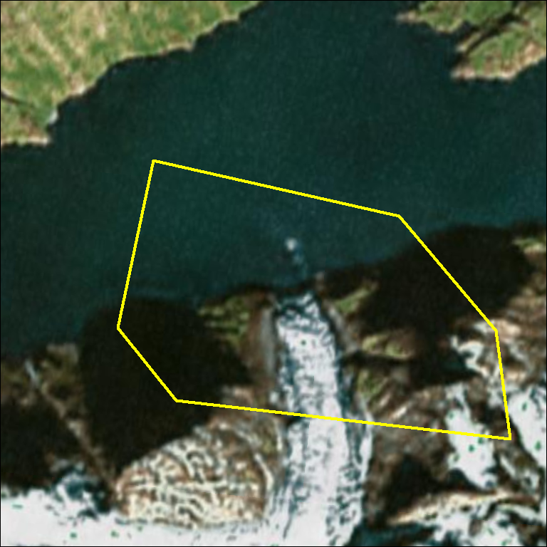
As this is a polar region, the ArcticDEM archive will likely have a large number of DEMs we can use, which we can identify from their extents, but how can we tell which have “good” data over this AOI without opening and viewing all of them in a GIS software? The valid_data.py script will allow us to do this. Say this is what one of the DEMs actually looks like:

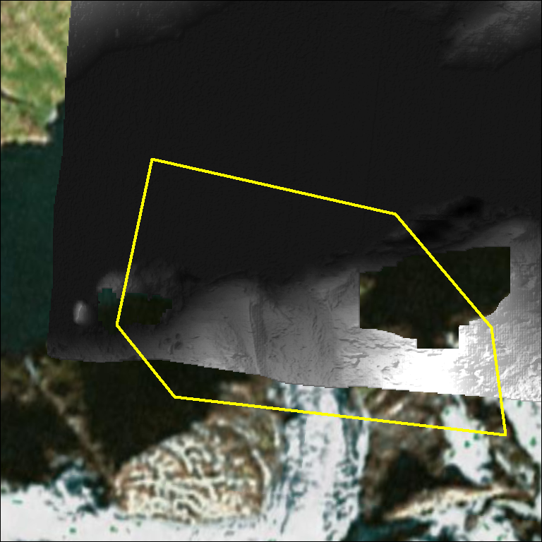
If we run the valid_data.py and write the output as a binary raster, we get:

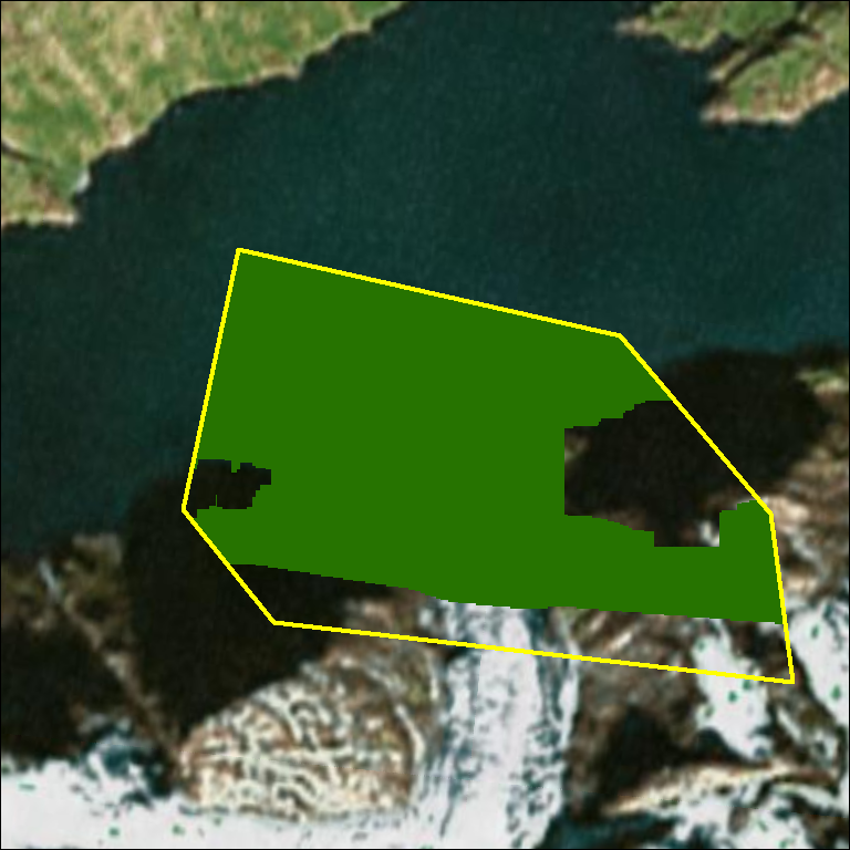
Which shows that while there are areas of missing data, we have valid data over our AOI. This binary raster will open much more quickly than the full resolution DEM and can also be used in subsequent selections.

The relevant function:

def valid_data(gdal_ds, band_number=1, write_valid=False, out_path=None):
    """
    Takes a gdal datasource and determines the number of
    valid pixels in it. Optionally, writing out the valid
    data as a binary raster.
    gdal_ds      (osgeo.gdal.Dataset):    osgeo.gdal.Dataset
    write_valid  (boolean)           :    True to write binary raster, 
                                          must supply out_path
    out_path     (str)               :    Path to write binary raster

    Writes 
    (Optional) Valid data mask as raster

    Returns
    Tuple:  Count of valid pixels, count of total pixels
    """
    # Get raster band
    rb = gdal_ds.GetRasterBand(band_number)
    no_data_val = rb.GetNoDataValue()
    arr = rb.ReadAsArray()
    # Create mask showing only valid data as 1's
    mask = np.where(arr!=no_data_val, 1, 0)
    # Count number of valid
    valid_pixels = len(mask[mask==1])
    total_pixels = mask.size
    
    # Write mask if desired
    if write_valid is True:
        if len(mask.shape) == 2:
            rows, cols = mask.shape
            depth = 1
        else:
            rows, cols, depth = mask.shape
        driver = gdal.GetDriverByName('GTiff')
        
        dst_ds = driver.Create(out_path, ds.RasterXSize, ds.RasterYSize, 1, rb.DataType)
        dst_ds.SetGeoTransform(ds.GetGeoTransform())
        out_prj = osr.SpatialReference()
        out_prj.ImportFromWkt(ds.GetProjectionRef())
        dst_ds.SetProjection(out_prj.ExportToWkt())
        for i in range(depth):
            b = i+1
            dst_ds.GetRasterBand(b).WriteArray(mask)
            dst_ds.GetRasterBand(b).SetNoDataValue(no_data_val)
        dst_ds = None

    return valid_pixels, total_pixels

Multi-Scale Topographic Position Index - TPI.py

A topographic position index (or TPI) is a derivative created from a digital elevation model. It describes the relative position of the terrain - is a given area higher than the area around it or lower than the area around it? TPI’s are useful for identifying ridges or depressions on the landscape. An application I have used TPI for is to identify slumps resulting from permafrost thaw, also known as thermokarst, specifically retrogressive thaw slumps.

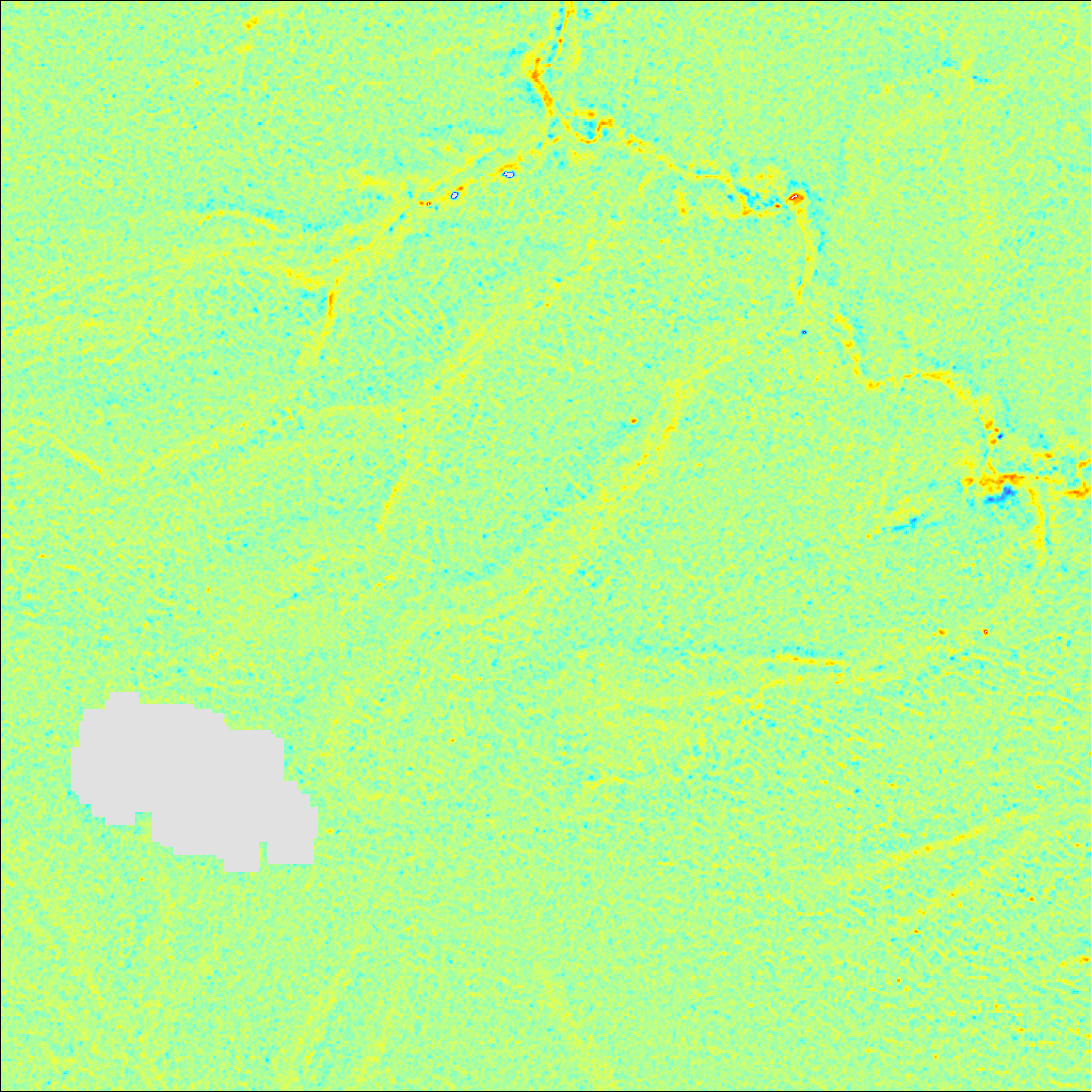
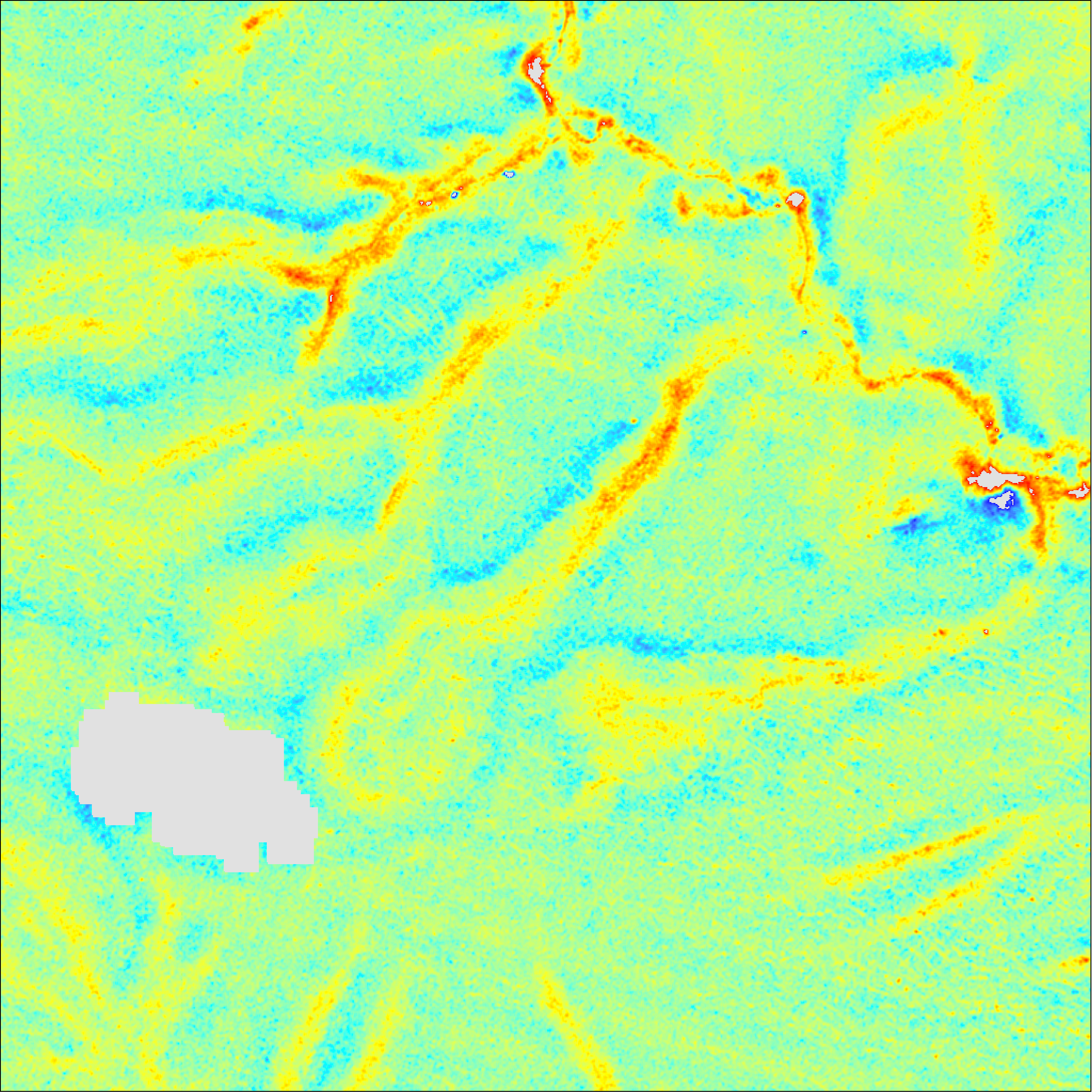
TPI’s are generated with a moving window kernel, which compares the elevation of each cell with the average elevation of a given number cells around it. The resulting TPI is highly dependent on the number of cells considered in the kernel. A smaller kernel size will show smaller scale depressions and hills. A larger kernel size will show larger features.

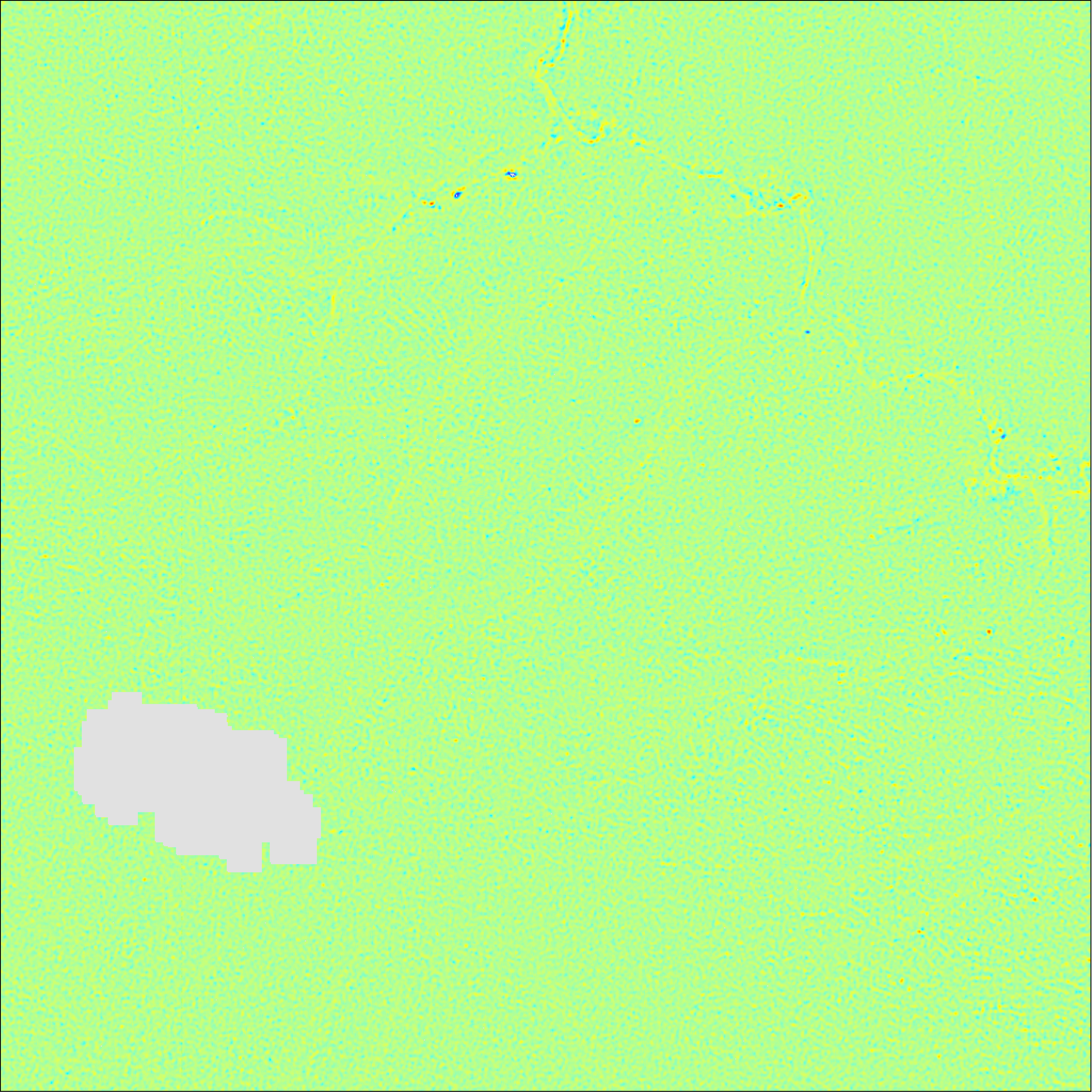
Thus it is critical to match the kernel size to the features of interest. I was unable to find a tool that had a configurable kernel size - most (GDAL, ArcMap, etc.) use a standard 3x3 kernel for all terrain indicies. So I wrote a script that would allow a user to vary the kernel size. Here are examples TPI’s generated from the same DEM showing a thermokarst thaw slump with differnt kernel sizes:
3x3:
21x21:
50x50:
100X100:

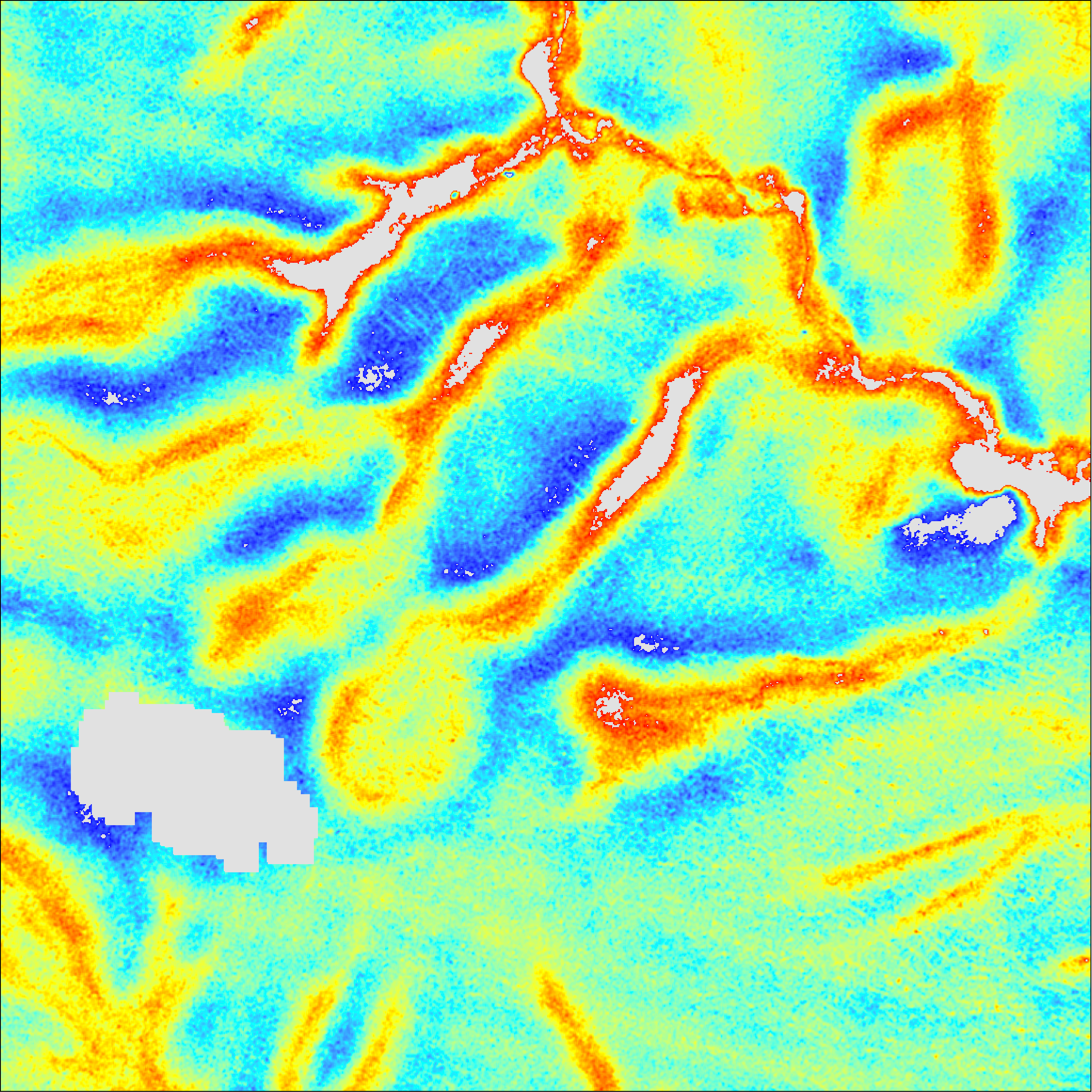
It is clear the different kernel sizes accentuate different features. This can be critical when creating a TPI to use in a feature identification workflow.